ECE 3310

Electrical Circuits: Laboratory

Signal Basics

©2008 by Professor Mohamad H. Hassoun

This Unit is intended as a review of the mathematics of functions (signals) and signal measurements.

Learning Objectives

By the end of this Unit, the student should have an understanding of the basic physical signals that are encountered in the study of electrical engineering. The following are specific learning objective:

· Identify a signal as sinusoid, exponential, square, or triangular from a given plot or function.

· Define the following terms: amplitude, peak-to-peak, period, frequency, average, RMS, duty cycle, rise time, fall time and decay constant.

· Define signal time-shift and amplitude shift (dc bias).

· Compute a signal’s amplitude, peak-to-peak, period, frequency, average, and RMS value, given the a signal’s analytical expression

· Measure a signal’s amplitude, peak-to-peak, period, frequency, average, RMS value and dc bias, given a plot of the signal (e.g., waveform displayed on an oscilloscope).

· Determine, experimentally and analytically, the duty cycle of a square wave.

· Determine, experimentally, the rise time and fall time of a pulse.

· Determine, analytically and experimentally, the phase shift between two sinusoidal signals.

· Determine, analytically and experimentally, the decay constant of an exponential signal.

Introduction

The study of time varying signals is of fundamental importance in engineering. Engineering students were introduced to signals (or functions) in high school and freshman college math courses. A signal is described by a function of the form y(x). For example, y(x) = x² + 1 represents a quadratic function (parabola). Here, x is referred to as the independent variable, and the value of y (the dependent variable) is determined by the value of x.

In engineering, functions where time is the independent variable are common. For example, in electrical engineering, time-dependent voltage, v(t), or current, i(t), signals are encountered in circuit analysis. Analog electronic circuits can be viewed as “signal processing” systems that transform one analog signal into another. Circuits are used to output a (processed) signal y_out(t) in response to an input signal y_in(t). The input signal could be a voltage signal generated by a function generator. The output could be a current through or voltage across a particular circuit component (say, a resistor, capacitor, or inductor).

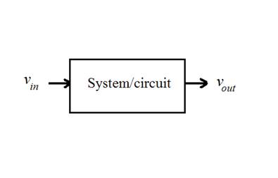
Figure 1 shows a circuit, and its corresponding block diagram. This circuit inputs the sinusoidal voltage signal v_in(t) and outputs the signal v_out(t). Towards the end of the Linear Circuits Analysis course, a student should be able to solve this circuit for all voltages and currents.

(a) (b)

Figure 1. An electric circuit (a) can be viewed as a system (b) that transforms one signal into another.

Figure 2. Input and response waveforms for the circuit in Figure 1.

For example, if the input signal is a cosine function with amplitude 12V and frequency 2rad/sec [i.e., v_in(t) = 12cos(2t)], the steady-state output signal (for the circuit in Figure 1) is v_out(t) = 8.37cos(2t - 0.95) Volts. The signals v_in(t) and v_out(t) are plotted in Figure 2. It is not difficult to see how the system/circuit has attenuated the input signal amplitude by about 30 percent [computed as 100*(8.37-12)/12)]; also, it has shifted the input signal by an angle of 54^o (computed as 0.95*180/p).

Basic Physical Signals

Physical signals are those signals that can be generated in the laboratory, experimentally, using physical devices. The basic physical signals encountered in the analysis of linear circuits are: constant (dc), sinusoid (ac), square, triangular and exponential (voltage and current) signal.

Constant Signal

A constant signal has the form y(t) = A, where A is a real-valued constant. As an example, Figure 3 shows a plot of the two constant signals y(t) = 5 and g(t) = -2.

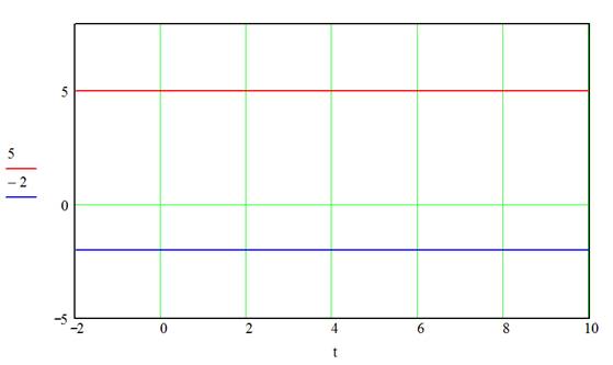
Figure 3. A plot of the signals y(t) = 5 and g(t) = -2.

Sinusoidal Signal

Sinusoidal signals are periodic signals of the form y(t) = Acos(wt + f), where the signal parameters A (amplitude) and w (frequency in rad/s) are positive real constants and f (phase or angle in rad) is a real constant. The sinusoidal signal may also be defined in terms of the sine function; note that Acos(wt) = Asin(wt + p/2). Figure 4 shows a plot of the signals y(t) = 3cos(2t + 1) and g(t) = 2sin(3t).

Figure 4. A plot of the signals y(t) = 3cos(2t + 1) and g(t) = 2sin(3t).

Periodic Square Signal

A periodic square signal consists of a train of pulses. The signal is defined in terms of an analytical expression, specified over one complete period. The following is an example of a repeating square signal whose plot is shown in Figure 5:

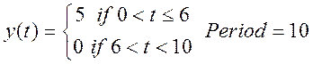
Figure 5. A plot of a square signal that repeats every 10 seconds.

Periodic Triangular Signal

Periodic triangular signals are repeating, piece-wise linear signals. They are defined in terms of an analytical expression, specified over one complete period. The following is an example of a repeating triangular signal whose plot is shown in Figure 6.

Figure 6. A plot of a triangular signal that repeats every 8 seconds.

Exponential Signal

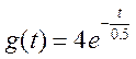
An exponential signal has the functional form: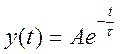, where A is a real-valued constant, and t is a positive-real constant (called the time constant). The time constant, t, determines the decay rate of y(t). Figure 7 compares the plots of 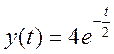and .

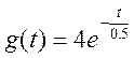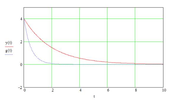
Figure 7. A plot of the signals 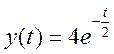and .

Signals with dc Bias

dc bias is achieved by adding a constant B to a signal y(t). This results in shifting all the values of y(t) by B, for all t. The plots of y(t) = 3cos(2t) and g(t) = 1 + 3cos(2t) are shown in Figure 8.

Figure 8. A plot of the signals y(t) = 3cos(2t) and g(t) = 1 + 3cos(2t ).

Time Shifted Signals

A signal may also be shifted in time by adding a constant a to the time variable t; i.e., y(t) is transformed into y(t + a). When a is negative (positive), the signal y(t + a) is shifted to the right (left). For example, consider the signal y(t) = 3cos(2t). Shifting t by -1 leads to y(t - 1) = 3cos[2(t - 1)] = 3cos(2t - 2). Note how the angle of a sinusoid is related to time-shift. Figure 9 compares y(t - 1) = 3cos(2t - 2) to y(t) = 3cos(2t).

Figure 9. A plot of the signals y(t) = 3cos(2t), and y(t - 1) = 3cos(2t - 2).

Signal Measurement Definitions

Important measurements of periodic signals are defined in this section. They include: amplitude, peak-to-peak, period, frequency, average, and RMS values. For square signals, the following measures are defined: duty cycle, rise time and fall time. The decay constant, a useful measure for exponential signals, is defined. Also, this section presents two methods for experimentally measuring the phase difference between two sinusoidal signals.

Amplitude

The amplitude of a pure sinusoidal signal (refer to Figure 10) is equal to its maximum value. Therefore, the amplitude of v(t) = Asin(wt) is A Volts.

Figure 10. Sine signal: y(t) = Asin(wt).

Peak-to-Peak Value

The peak-to-peak voltage, V_PP, is defined as the difference between the maximum and the minimum values of the signal. For example, V_PP = 2A for the signal y(t) = Asin(wt).

Period and Frequency

The period, T, of a repetitive signal is defined as the time it takes for the signal to undergo one complete cycle (refer to Figure 10). The frequency, f, of a signal is the number of cycles per second. In other words, f = 1/T cycles/sec, or Hz. f is referred to as the Hz-frequency. The radian frequency of a signal is defined as w = 2pf rad/sec. As an example, the signal y(t) = 3cos(2t) has w = 2 rad/sec, f = w/2p = 2/2p = 0.3183 Hz and a period T = 1/f = 3.1415 sec.

Average Value

The average of a periodic signal y(t) is defined as

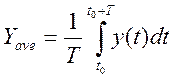(1)

where t₀ is any constant (including 0) and T is the period. Equation (1) suggests that the average value can be determined (by inspection, if possible) as the “area under the curve” of one signal period divided by T. For example, the average of the signal y(t) = Asin(wt) is zero since the area under the curve is zero.

RMS Value

RMS value (also known as the effective or dc value) is the root-mean-square value of the signal. For a periodic signal y(t), the RMS value, Y_rms, is defined as

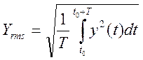(2)

A voltage signal v(t) placed across a resistor R, delivers an average power equal to ; this is the same power that a constant voltage signal (dc voltage) would have delivered to the resistor. Therefore, the RMS value is also called the effective or dc value of the signal. Note that the RMS value for a constant signal, y(t) = B, is B.

For pure sinusoidal signals of the form v(t) = Acos(wt + f), the RMS value is equal to 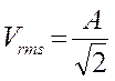. Note that the RMS value is not affected by the frequency or phase (time-shift) of the signal. The sinusoidal voltage signal delivered by a house’s electric outlet is rated at 120Volts. This is the RMS value of the voltage signal. Since the frequency is 60 Hz, one can write the expression for the voltage signal as Volts. This can be verified by plugging v(t) in Equation (2), to obtain (employing Mathcad software):

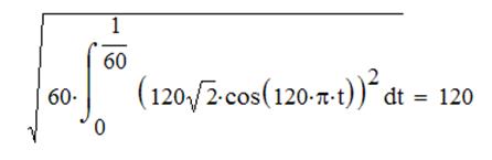
The signal v(t) and its RMS value are shown in Figure 11.

Figure 11. Voltage signal from a house’s electric outlet and its RMS value.

Bias Effects on Average and RMS Values

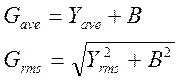
Given the signal y(t) and its average value, Y_ave, and RMS value, Y_rms. How does adding a constant B to y(t) affects the average and RMS values of the biased signal? Let the biased signal be g(t) = y(t) + B. It can be shown that the biased signal average and RMS values are given by

Duty Cycle

Consider a pulse train (square) signal with period T. The duty cycle is the ratio of the pulse width (Width, refer to Figure 12) to the period, expressed as a percentage:

Duty cycle = 100*(Width)/T

Figure 12. Pulse width of a triangular signal

Rise Time and Fall Time

The rise time and fall time of a pulse are depicted in Figure 13. The dashed horizontal lines represent the 10% and 90% of the signal’s peak-to-peak value. The rise time is the time it takes the rising edge of the pulse to go from the 10% threshold to the 90% threshold. Similarly, the fall time is the time it takes the falling edge of the pulse to go from 90% to 10% threshold. Generally speaking, the rise time is not equal to the fall time.

Figure 13. Rise time and fall time of a signal

Time Constant

The exponentially decaying signal of the form appears in the natural response of all RC and RL circuits. For example, in a parallel RC circuit where the capacitor has an initial voltage V₀, the resistor (and capacitor) voltage decays as 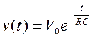, for t > 0. The product of RC has the unit seconds, and it controls the rate at which the voltage decays. In circuit textbooks, the constant RC is renamed as t (the circuit time constant).

Figure 7 (see above) show plots of for A = 4 and t = 0.5 and 4. The larger the time constant is, the slower the rate of decay. When t = 0, the signal value is A. When t = t, the signal value drops to A/e = 0.368A, or about 63.2 percent of the value of the signal at t = 0. Therefore, the time constant (of an exponentially decaying signal) is defined as the time it takes the signal to drop by 63.2 percent of its initial value, at t = 0. Given a graph of , one can employ this definition to approximate the time constant (Problem 5). See Problem 6 for an alternative graphical method for estimating t.

It should be noted that the signal drops by over 99 percent after 5 time constants; 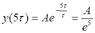= 0.0067A, which corresponds to 99.33% of A.

Phase Difference

In practice, one could use an oscilloscope to display and compare two voltage signals. When dealing with steady-state RLC circuits under sinusoidal input, say v_in(t) = Vcos(wt), all voltages and currents in the circuit have the functional form y(t) = Acos(wt - f). The angle constant f (measured in radians) is the phase shift between the response signal and the input signal.

The angle f can be transformed to reflect the amount of time shift between the signals y(t) and v_in(t). The signal y(t) = cos(wt - f) can be rewritten as y(t) = cos[w(t - f /w)]. If we define the signal g(t) = cos(wt) as a reference signal, then y(t) = g(t - f /w). In other words, y(t) is obtained by time shifting the reference signal g(t) by f /w seconds. When f is positive, the waveform of y(t) is (delayed) shifted to the right of g(t).

The above analysis suggests a method for measuring the phase difference between two sinusoids (of equal frequency) acquired by a two channel oscilloscope. First, one of the signals is used to measure the period T. Next, the scope’s X-cursor is used to find the time difference between the t-intercept of one signal and the closest t-intercept of the second signal. Let the difference be Dt. Finally, the phase difference is computed as f =w Dt = 2pDt/T radians, or f = 360Dt/T degrees. For example, the phase difference between the two signals in Figure 14 is f = 2pDt/T = (2p)(0.5- 0.25)/(0.24 - (- 0.76)) = 1.57 rad (or about 90 degrees). We measured the phase of the “dotted-line” signal with respect to the “solid-line” signal. In other words, the solid-line signal is our reference signal. The solid-line signal is g(t) = cos(2pt), and the dotted-line signal is y(t) = cos(2pt – 1.57). We say that y(t) is delayed by 0.25 sec relative to g(t). We may also say that y(t) lags g(t) by about 90 degrees.

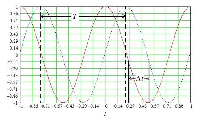
Figure 14. Approximating the phase difference between two sinusoids.

The Lissajous method may also be used to measure the phase difference between two sinusoidal signals of the same frequency and amplitude. This method assumes that an oscilloscope, operating in the XY mode, is used to acquire the signals. Here, one signal is connected to Channel 1 of the scope, and the second signal is connected to Channel 2. The displayed waveform (an ellipse, see Figure 15) should be centered (using the vertical position knobs) at the display’s center point. The phase difference can now be computed as (in reference to the labeled distances in Figure 15): f = sin^-1(C/D).

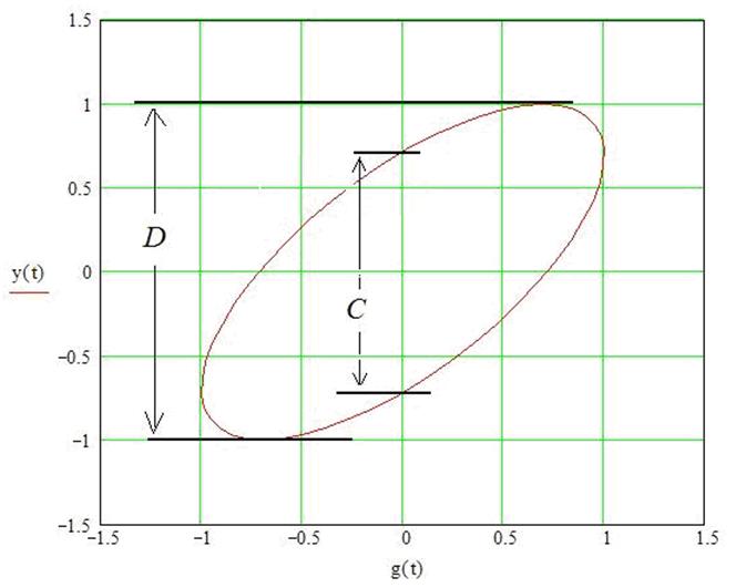
Figure 15. Measuring phase difference using the Lissajous method.

Pre-Lab Activity (Experiment 2)

1. Determine the average, RMS, and duty-cycle values for the signal in Figure 5.

2. Determine the peak-to-peak, average and RMS values for the signal in Figure 6.

3. Show that the RMS value for the signal y(t) = Asin(wt) + B is given by

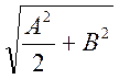
Now, find the RMS value for the signal y(t) = 5sin(wt) + 2 and compare it to the sum of the individual RMS values of the signals g(t) = 5sin(wt) and h(t) = +2.

4. The rising edge of a pulse signal is shown below. Determine the rise time.

5. Employ the following plot of an exponential signal to approximate the signal’s time-constant.

6. Show that 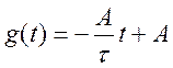is the equation of the line tangent to the function 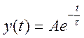at t = 0. Show that the line intersects the t-axis at t = t. This suggests a two-step graphical method for determining the time constant t: (1) Draw a line tangent to y(t) at the point (0, A), then (2) t is the point at which this line intersects the time axis. Employ the tangent line method to estimate t for the function y(t) in Problem 5.

7. Employ the following plot of two sinusoidal signals to approximate the difference in phase (angle) between g(t) and y(t). Give your answer in degrees.

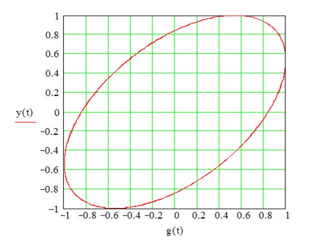
8. Employ the following plot of two sinusoidal signals [plotted as y(t) vs. g(t)] to approximate the difference in phase between the signals. Give your answer in degrees.

9. It can be shown that the sum of two sinusoids, Acos(wt) + Bsin(wt), is equal to Ccos(wt + f) where,

Express the signal cos(2t) + 2sin(2t) as Ccos(wt + f). Check your answer by comparing the plots of the two signals: cos(2t) + 2sin(2t) and Ccos(wt + f). Verify that both signals have the same RMS value.