Taylor Series
Functions of
single variable case:
Consider a
function of one variable F(x), where x is a scalar parameter we are adjusting. We will assume that F(x)
is an analytic function, so that all of its derivatives exist. Then F(x)
can be represented by its Taylor series expansion about some nominal point x*:
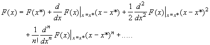
We will use the Taylor series expansion to approximate the F(x), by limiting the expansion to a finite number of terms.
Example:
Consider the function F(x)
= cos(x). The following is the Taylor
series expansion for F(x) about the point x* = 0:

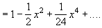
The zeroth-order
approximation of F(x) is

The second-order
approximation is

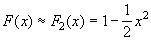
(Note that in this case the
first-order approximation is the same as the zeroth-order approximation, since
the first derivative is zero).
The fourth-order
approximation is
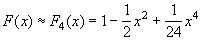
Let us employ Matlab to
compare F(x) to its approximations of various order:
for x = -6:0.05:6
k=k+1;
y(k)=x;
F(k)=cos(x);
F0(k)=1;
F2(k)=1-0.5*x^2;
F4(k)=1-0.5*x^2+(1/24)*x^4;
end
plot(y,F,y,F0,y,F2,y,F4)
axis([-6 6 -1.5 1.5])
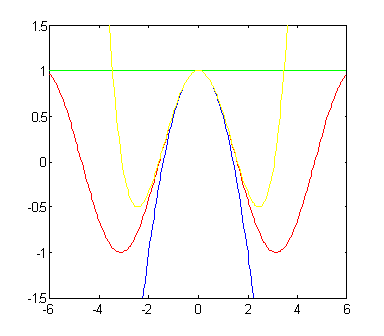
F F0 F2 F4
Next, Matlab
"taylor" command is utilized to generate the power series for cos(x):
1-1/2*x^2+1/24*x^4+O(x^6)
Note
that the default here is to compute the first 6 terms in the expansion and to
expand at x* = 0. Here is an
expansion using eight terms
1-1/2*x^2+1/24*x^4-1/720*x^6+O(x^8)
Let us generate plots of cos(x) and its approximation:
g='1-1/2*x^2+1/24*x^4-1/720*x^6';
fplot(y1,[-6 6 -1.5 1.5])
hold
fplot(g, [-6 6 -1.5 1.5], '-b')

We will use
Taylor series approximation of objective functions to investigate the shape of
the objective function in the neighborhood of possible optimum points (extreme
points: minima/maxima).
Functions of
multiple variables case:

The following expression
extends the Taylor series expansion to functions of n variables:
 =

+ + ….
Where  is the gradient of F(x)
evaluated at x*
and  is the Hessian of F(x) evaluated at x*
Here:


and

A sufficient condition for
an extreme point x* (i.e.,  F(x*) = 0) to be a minimum is to have a positive
definite Hessian at x* (i.e.,
 has positive (nonzero) eigenvalues.
Example:
Consider a function of two
variables
F(x) = F(x1, x2) = (x2
- x1)4 +8x1x2 - x1
+ x2 + 3
1.
Find
all extreme (stationary) points.
2.
Test
extreme points to determine all minima.
3.
Find
the second-order Taylor series expansion at each minima.
4.
Plot
F(x) and the two Taylor series expansions in part 3.
Solution:
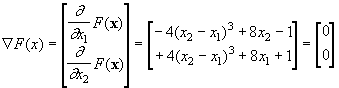
This function has the
stationary points:
x1=[-0.42 0.42]T, x2=[-0.13 0.13]T,
and x3=[0.55 -0.55]T
which are determined as
solutions to the equation 
Next we test the stationary
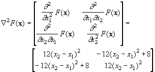
points x* for minima. A sufficient
condition is that the Hessian of F at
a minimum is positive definite. So, let us compute the Hessian matrix:
To test the definitness of this matrix we can check the eigenvalues. If the eigenvalues
are all positive, the Hessian is positive
definite, which guarantees a strong minimum.
If we evaluate the Hessian
at x1=[-0.42 0.42]T,
we find
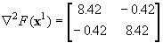 .
The eigenvalues are the
solution of the quadratic equation (characteristic equation) obtained from:

Solving we get l1 = 8.84, l2 = 8.0, therefore x1 is a strong minimum.
Similarly, the eigenvalues
of the Hessian at x3=[0.55
-0.55]T are l1 = 21.42, l2 = 8.0, therefore x3 is a strong minimum.
On the other hand, the
eigenvalues of the Hessian at
x2=[-0.13 0.13]T
are l1 = -6.26, l2 = 8.0, therefore x2 must be a saddle point.
Let us now approximate the
function F at its the two minima x1=[-0.42 0.42]T
and x3=[0.55 -0.55]T employing second-order
Taylor series expansion:
Noting that for the minima
at x1=[-0.42 0.42]T, the gradient is zero and F(x1)
= 2.93 (by direct substitution). The Hessian at x1 has already been evaluated above. Here is the
expansion:
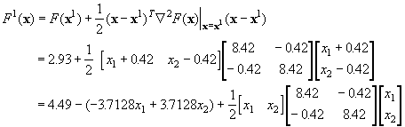
Repeating this process for x3 results in

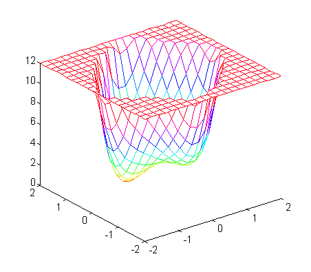
The following are plots of
the original function F(x) and its two approximations F1(x) and F3(x).
Matlab Program to generate plots
for x1=-2:0.2:2
i=i+1;
x(i)=x1;
j=0;
for x2=-2:0.2:2
j=j+1;
y(j)=x2;
F(i,j)=(x2-x1)^4+8*x1*x2-x1+x2+3;
if F(i,j) > 12,
F(i,j) = 12;
end
end
end
mesh(x,y,F)
axis([-2 2 -2 2 0 12])
Plot
for F1
i=0;
for x1=-2:0.2:2
i=i+1;
x(i)=x1;
j=0;
for x2=-2:0.2:2
j=j+1;
y(j)=x2;
F1(i,j)=4.49-(-3.7128*x1+3.7128*x2)+0.5*[x1
x2]*H1*[x1 x2]';
if F1(i,j) > 12,
F1(i,j) = 12;
end
end
end
mesh(x,y,F1)
axis([-2 2 -2 2 0 12])

Plot
for F3
H3=[14.71 -6.71; -6.71
14.71];
i=0;
for x1=-2:0.2:2
i=i+1;
x(i)=x1;
j=0;
for x2=-2:0.2:2
j=j+1;
y(j)=x2;
F3(i,j)=7.41-(11.781*x1-11.781*x2)+0.5*[x1
x2]*H3*[x1 x2]';
if F3(i,j) > 12,
F3(i,j) = 12;
end
end
end
mesh(x,y,F3)
axis([-2 2 -2 2 0 12])
